Data Structure and algorithms
- Complexity
- Linear structures
- Tree structures
- Other common data structures
- Search algorithms
- Sorting algorithms
Complexity
Array
fixed length, indexable, should shift after insertions and deletions

Array Operation
Insertion O(n)
- insert an element in the specified index
- shift the subsequent item to the right
Deletion O(n)
- delete the specified element
- shift the subsequent item to the left
Searching in a sorted array
Linear search
Best case-O(1)
Worst case-O(n)
Average case-O(n/2)->O(n)
Binary search O(logn)
Sorting array

Stack
Last In First Out
Stack Operation
Push(S,x): insert x to the top of the stack S
Pop(S): extract the top of the stack S
Top(s): return the topmost element of stack S without removing it
isEmpty(s): return whether the stack S is empty
Implementation
Array
Push() O(1)
1 | if s.top=s.len |
Pop() O(1)
1 | if isEmpty(s) |
Top() O(1)
1 | if isEmpty(s) |
isEmpty() O(1)
1 | if s.len=0 |
Search O(n)
Use stack implements a simple calculator
- transfer to postfix notation
3-2-1>>32-1-
3-2*1>>321*-
- use stack to calculate
3-2-1>>32-1-
1 | push(3) |
- exercise
10 + (44 − 1) * 3 + 9 / 2
((1 - 2) - 5) + (6 / 5)
(((22 / 7) + 4) * (6 - 2))
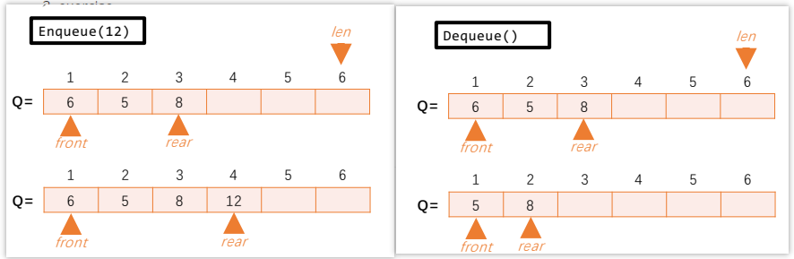
Queue
First In First Out
Operation
Enqueue(Q,x): put an element x at the end of queue Q
Dequeue(Q): extract the first element from queue Q
Implementation
Array 1
Enqueue in the tail -O(1)
Dequeue in the position0 -O(n)
Array 2
Enqueue in the position0 -O(n)
Dequeue in the tail -O(1)

Array 3 -Circular queue
Enqueue: O(1)
Dequeue: O(1)
Peeking (get the front item without removing it) O(1)
isFull: O(1)
isEmpty: O(1)
search: O(n)
algorithm implement
Data members:
• Q: an array of items • Q.len: length of array • Q.front: position of the front item • Q.rear: rear item position + 1 (not an item)
Enqueue
1 | if isFull(Q) |
Dequeue
1 | if isEmpty(W) |
isFull and isEmpty

Linked List

Node: An object containing data and pointer(s) Pointer: Reference to another node Head: The first node in a linked list Tail: The last node in a linked list

No limited to size
require more space per element
Initial
...
Operation
print
insert
Delete
Hash table
Dictionary ADT
key:value
implement of ADT
array
Space usage: O(n)
Search usage: O(n)
| Array index | Key | Value |
|---|---|---|
| 0 | 3 | Coffee |
| 1 | 15 | Bread |
| 2 | 8 | Tea |
Large array
Space usage: O(U)-max key
Search usage: O(1)
| Array index | Key | Value |
|---|---|---|
| ... | ... | ... |
| 3 | 3 | Coffee |
| ... | ... | ... |
| 8 | 8 | Tea |
| ... | ... | ... |
| 15 | 15 | Bread |
Hash table
Converts a key (of a large range) to a hash value (of a small range). e.g. k mod m
Space usage: O(n)
Search usage: O(1)
Collision solution
collision: different keys have the same hash value
Chaining
use a linked list

load factor
\[ \lambda = \frac{n}{m} \]
n is the number of keys, m is the total number of buckets.
Measures how full the hash table is
it is suggested to keep \(\lambda\) < 1
cost
time
cost of search: O(1)+O(l), l is the length of the linked list
worst case: O(1)+O(n)
Average case: O(1)+O(\(\lambda\))
space
requires additional space to store the pointers in linked lists of entries.
Worst case: n-1 additional space
Average case: \(\lambda\)-1 additional space
Opening addressing: probing
Insert

Search

Delete

Load factor
must \(\lambda < 1\)
How to deal with the hash table when ! becomes large?
- Make a large hash table and move all elements into it.
- Simply add an additional hash table
probing type
Linear probing
\[ H(k,i) = (H_0(k) + i)\space mod \space m \] have clustering problem, multiple keys are hashed to consecutive slots.
performance degrade significantly when \(\lambda\)> 0.5.
Quadratic probing \[ H(k,i) = (H_0(k) + a\cdot i+b\cdot i^2)\space mod \space m \] reduces the clustering problem.
string key

Tree
a tree is an abstract model of a hierarchical structure consists of a set of nodes and a set of edges.
Every node except the root has exactly one parent node.
Definition
Length of a path: The number of edges in the path.
The height of a node:
The largest path length from that node to any leaf node (not including ancestors).
Each leaf node has the height 0.
The height of a tree: The maximum level of a node in a tree is the tree’s height.
The depth of a node:
The node's level (depth) of a node is the length of the path from that node to the root.
The depth of the root is zero.
Binary Tree
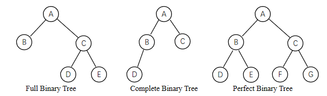
Full Binary Tree
Every node has either 0 or 2 children.
Complete Binary Tree
Every level, except the last level, is completely filled, and all nodes in the last level are as far left as possible (left justified).
Perfect Binary Tree
Every node except the leaf nodes have two children and every level is completely filled.

list representation: [Root, left-sub-tree, right-sub-tree]
Binary Search Tree
Insertion - O(h)
Search - O(h)
Deletion: O(h)
ℎ is O(logn) if tree is balanced.
all is O(n) in worst case
左小右大
Search Operation
1 | Algorithm SearcℎBST(t, target) |
Insert
average case: O(n) = logn
worst case: O(n) = n
1 | Algorithm Insert(t, node) |
find minimun
O(h)-ℎ is the depth of the tree
1 | Algorithm Minimum(t) |
Deletion in BST
has no child
delete the node
has one child
use the child to replace z
has two children
delete the minimum node x of the right subtree of z (i.e., x is the successor of z), then replace z by x.

Tree Traversal
Depth-first Tree Traversal
implement: stack
preorder 前序
1 | def preorder(root): |
postorder 后序
1 | def postorder(root): |
inorder 中序
1 | def inorder(root): |
Breadth-first Tree Traversal
implement: queue
1 | def bfs(root): |
Sorting
stable, unstable, inplace, outplace

Selection sort


time-\(O(n^2)\)
in-place
unstable
1 | def selection_sort(arr): |
Insertion Sort

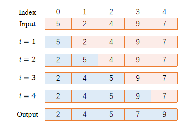
time -\(O(n^2)\)
in-place
stable
1 | def insertionSort(arr): |
Merge Sort
time - O(nlogn)
not in-place
stable
- Divide: divide the array A into two sub-arrays (L and R) of n/2 numbers each.
- Conquer: sort two sub-arrays recursively.
- Combine: merge two sorted sub-arrays into a sorted array.

1 | Algorithm MergeSort(A, n) |
Merge function - O(n)
1 | Algorithm Merge(A, n_A,B,n_B,C) |
Quick Sort
O(nlogn)
in-place