NGCF

Posted on 2023-02-24 Edited on 2024-06-19 In RecSys

Background

question: example(the Laplacian)

Some Definition

Recommendation system: Estimate how likely a user will adopt an item based on the historical interaction like purchase and click.
Collaborative filtering(CF): behaviorally similar users would exhibit similar preference on items.

CF consists of
1. embedding: transforms users and items into vectorized representations. e.g. matrix factorization(MF),deep learning function...
2. interaction modeling: reconstructs historical interactions based on the embeddings. e.g. inner product, neural function...
collaborative signal: signal latent in user-item interactions

Existing Problem

The current embedding process of CF doesn't encode a collaborative signal. Most of them focus on the descriptive feature(e.g. user id, attributes). When the embeddings are insufficient in capturing CF, the methods have to rely on the interaction function to make up for the deficiency of suboptimal embeddings

Main contribute

Highlight the critical importance of explicitly exploiting the collaborative signal in the embedding function of model-based CF methods.
Propose NGCF, a new recommendation framework based on a graph neural network, which explicitly encodes the collaborative signal in the form of high-order connectivities by performing embedding propagation.

Model

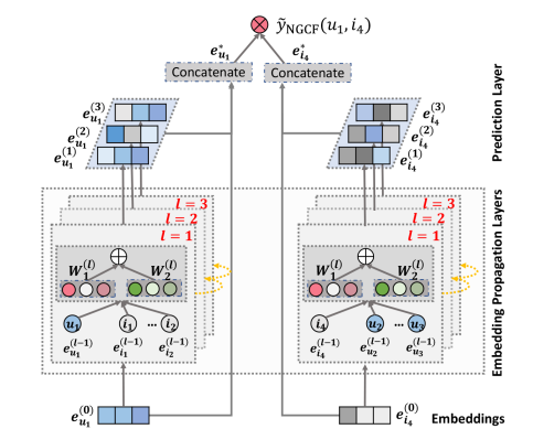
There are three components in the framework:

Embedding layer: offers and initialization of user embeddings and item embeddings;
Multiple embedding propagation layers: refine the embeddings by injecting high-order connectivity relations;
Prediction layer: aggregates the refined embeddings from different propagation layers and outputs the affinity score of a user-item pair.

Embedding layer

Just initializing user embeddings and item embeddings by using ID or other features.

Get user embedding $e_i$ and item embedding $e_u$.

Multiple Embedding Propagation Layers

One layer propagation

It consists of two parts: Message Construction and Message aggregation.

Message Construction

$m_{u<-i}$: the result of the message construction module. It is a message embedding that will be used to update the target node.

$e_i$: Embedding of neighbor item.

meaning : encode neighbor item's feature.

$e_i⊙e_u$ : element-wise product of $e_i$ and $e_u$.

meaning: encodes the interaction between $e_i$ and $e_u$ into the message and makes the message dependent on the affinity between $e_i$ and $e_j$.

$W_1$, $W_2$: trainable weight matrices， the shape is ($d'$, $d$), while $d$ is the size of the initial embedding, $d'$ is the size of transformation size.

$P_{ui}$: to control the decay factor on each propagation on edge (u, i). Here, we set $P_{ui}$ as Laplacian norm $ $, $ N_u$, $ N_i$ is the first-hot neighbors of user u and item i. (就是拉普拉斯矩阵归一化！！$D^{-\frac{1}{2}}AD^{-\frac{1}{2}}$)

meaning -From the viewpoint of representation learning: $P_{ui}$ reflects how much the historical item contributes to the user preference.

From the viewpoint of the message passing: $P_{ui}$ can be interpreted as a discount factor, considering the messages being propagated should decay with the path length.

Message Aggregation

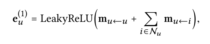
$e_u^{(1)}$: the representation of user u after 1 propagation layer.

$m_{u<-u}$: self-connection of u. Here is $W1e_u$.

meaning: retain information of original feature.

$m_{u<-i}$： neighbor node propagation.

High-order propagation

Formulate Form

By stacking l-embedding propagation layers, a user (and an item) is capable of receiving the messages propagated from its l-hop neighbors. The formulates are similar to one-layer propagation.

Matrix Form

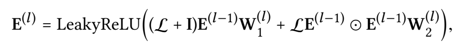
$E^{(l)}$ : the representations for users and items obtained after l-layers propagation. Shape is (N+M,d)

L: Laplacian matrix for the user-item graph.

D is the diagonal degree matrix. where $D_{tt}=\vert N_t\vert$ meaning the D[t][t] is the number of neighbors' node. The shape is (N+M, N+M), because there are totally n+m node(including user and item)

A is the adjacency matrix. The shape of R is (N, M), while the shape of A is (N+M, N+M).

some extra knowledge: 理解拉普拉斯矩阵

I: identity matrix

A simple example for matrix form:

Suppose we have 2 users (A, B), 3 items(C, D, E), N=2 and M=3.

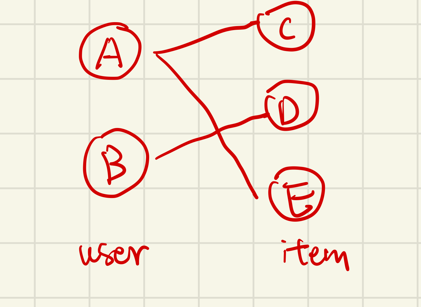
D9B00E7DDF74FF18B83E42668335328A

Let consider this part: $(L+I)E^{(l-1)}W^{(l)}$

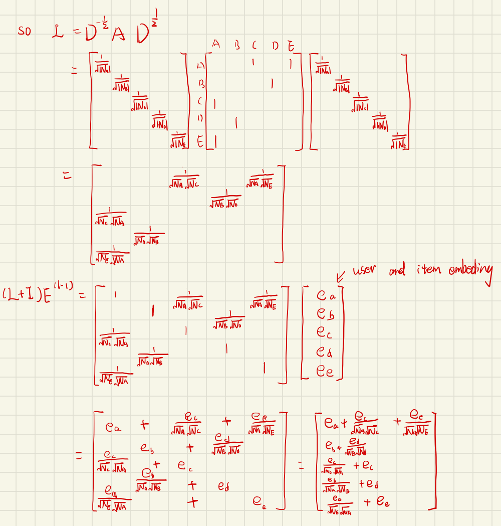
After calculating $(L+I)E^{(l-1)}$, we get information on self-connection and neighbor-propagation (after the Laplacian norm), and then we can multiply the trainable parameter W1(MLP).

拉普拉斯矩阵归一化的不成熟小理解：

①target node由n个邻居点做贡献，为了避免邻居越多，target node的value越大的情况，首先除$\frac{1}{\sqrt{N_n}}$, 大概也可以理解为邻居越多，每个邻居对其造成的影响越小

②只做一次norm影响对称性，所以为了保持对称性在做一次$\frac{1}{\sqrt{N_t}}$,可以理解为neighbor node有多少邻居对他给到每个邻居的权重有影响，是否能理解为邻居越多说明这个node能提供的信息更普通没价值（例如所有用户购买了水，对推荐系统来说，水能提供的信息就没那么有用）

xxxxxxxxxx class UV_Aggregator(nn.Module): """ item and user aggregator: for aggregating embeddings of neighbors (item/user aggreagator). """ def init(self, v2e, r2e, u2e, embed_dim, cuda="cpu", uv=True): ... def forward(self, nodes, history_uv, history_r): # create a container for result, shpe of embed_matrix is (batchsize,embed_dim) embed_matrix = torch.empty(len(history_uv), self.embed_dim, dtype=torch.float).to(self.device) # deal with each single item nodes' neighbors for i in range(len(history_uv)): history = history_uv[i] num_histroy_item = len(history) tmp_label = history_r[i] # e_uv : turn neighbors(user node) id to embedding # uv_rep : turn single node(item node) to embedding if self.uv == True: # user component e_uv = self.v2e.weight[history] uv_rep = self.u2e.weight[nodes[i]] else: # item component e_uv = self.u2e.weight[history] uv_rep = self.v2e.weight[nodes[i]] # get rating score embedding e_r = self.r2e.weight[tmp_label] # concatenated rating and neighbor, and than through two layers mlp to get fjt x = torch.cat((e_uv, e_r), 1) x = F.relu(self.w_r1(x)) o_history = F.relu(self.w_r2(x)) # calculate neighbor attention and fjt*weight to finish aggregation att_w = self.att(o_history, uv_rep, num_histroy_item) att_history = torch.mm(o_history.t(), att_w) att_history = att_history.t() embed_matrix[i] = att_history # result (batchsize, embed_dim) to_feats = embed_matrix return to_featspython

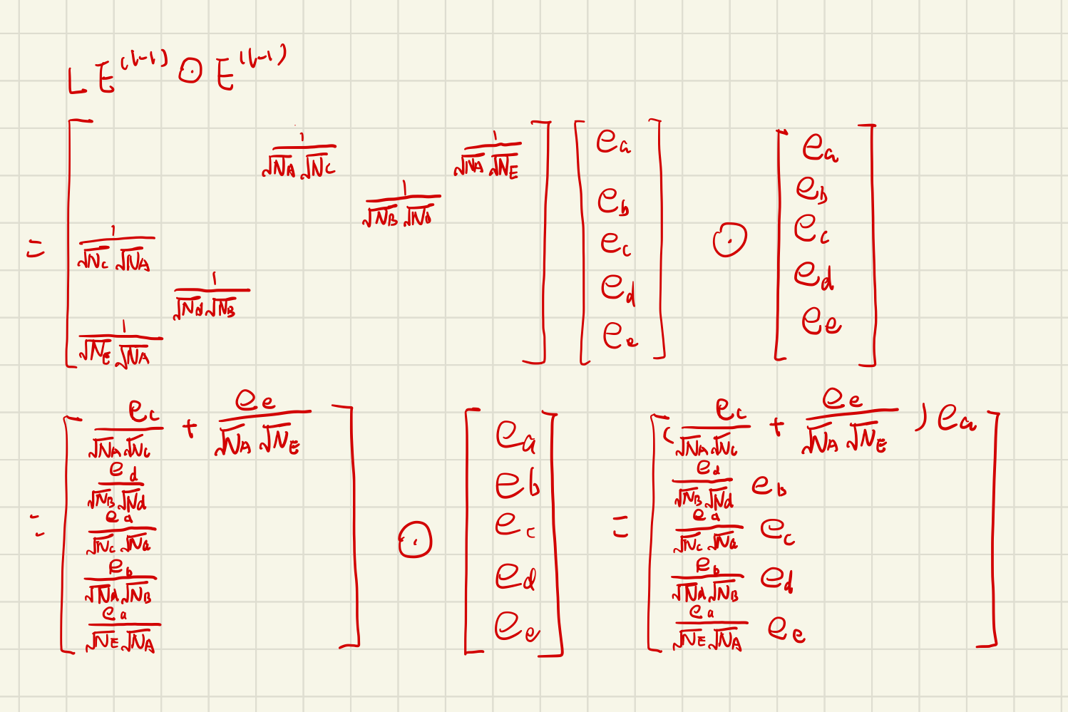
We get information on the interaction between $e_i$ and $e_u$ (after the Laplacian norm), and then we can multiply the trainable parameter W2(MLP).

Add two parts and through LeakyRelu, we get user or item embedding after l-layers propagation.

Model Prediction

Just concatenate all propagation layers' output embedding, and use inner product to estimate the user's preference towards the target item.

Optimization

Loss

BPR Loss: assumes that the observed interactions, which are more reflective of a user’s preferences, should be assigned higher prediction values than unobserved ones.

Optimizer: Adam

Model Size

In NGCF, only W1 and W2 in the propagation layer need to be trained, so has $2Ld_ld_{l-1}$ more parameters, while L is always smaller than 5 and $d$ is set as the embedding size(e.g. 64) which is also small.

Message and Node Dropout

Message dropout: randomly drops out the outgoing messages (equal to dropout edge).

meaning: endows the representations more robustness against the presence or absence of single connections between users and items.

example: For the $l-th$ propagation layer, we drop out the messages being propagated, with a probability $p1$.
Node dropout: randomly blocks a particular node and discards all its outgoing messages.

meaning: focuses on reducing the influences of particular users or items.

example: For the $l-th$ propagation layer, we randomly drop $(M + N)p2$ nodes of the Laplacian matrix, where $p2$ is the dropout ratio.

区别：对于message dropout，计算时node的邻居数、拉普拉斯norm都是正常的，就是更新embedding的时候遗漏了信息，作用是提高一下鲁棒性和容错性；对于Node dropout，直接在拉普拉斯矩阵中屏蔽若干个node，可能影响临界点数、归一化数值等，在矩阵运算时候就有影响，作用是希望模型不要过于依赖某些特定邻接点，没了部分点依然能正常运行。

Experiment

Conclusions from comparing with other models

The inner product is insufficient to capture the complex relations between users and items.
Nonlinear feature interactions between users and items are important
Neighbor information can improve embedding learning, and using the attention mechanism is better than using equal and heuristic weight.
Considering high-order connectivity or neighbor is better than only considering first-order neighbor.
that exploiting high-order connectivity greatly facilitates representation learning for inactive users, as the collaborative signal can be effectively captured. And the embedding propagation is beneficial to relatively inactive users.

Study for NGCF

....

Effect of High-order Connectivity

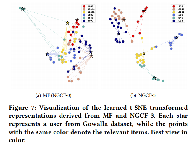
the representations of NGCF-3 exhibit discernible clustering, meaning that the points with the same colors (i.e., the items consumed by the same users) tend to form the clusters.
when stacking three embedding propagation layers, the embeddings of their historical items tend to be closer. It qualitatively verifies that the proposed embedding propagation layer is capable of injecting the explicit collaborative signal (via NGCF-3) into the representations.