KGAT
.
Background
利用KG作为辅助信息,并将KG与user-item graph 整合为一个图
Background

Previous model:
CF: behaviorally similar users would exhibit similar preference on items.
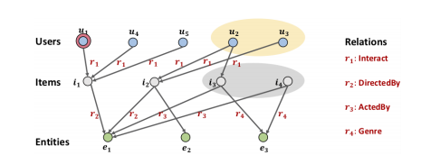
focus on the histories of similar users who also watched \(i1\), i.e., \(u4\) and \(u5\);
SL: transform side information into a generic feature vector, together with user ID and item ID, and feed them into a supervised learning (SL) model to predict the score.
emphasize the similar items with the attribute \(e1\), i.e.$ i2$.
current problem:
existing SL methods fail to unify them, and ignore other relationships in the graph:
- the users in the yellow circle who watched other movies directed by the same person \(e_1\).
- the items in the grey circle that share other common relations with \(e_1\).
User-Item Bipartite Graph: \(G_1\)
\[ \{(u,y_{ui},i)|u\in U, i\in I\} \] \(U\): user sets
\(I\): item sets
\(y_{ui}\): if user \(u\) interacts with item \(i\) \(y_{ui}\)=, else \(y_{ui}\)=0.
Knowledge Graph \(G2\)
\[ \{(h,r,t)|h,t\in E, r\in R\} \]
\(t\) there is a relationship \(r\) from head entity h to tail entity \(t\).
\(CKG\): Combination of \(G1\) and \(G2\)
- represent each user-item behavior as a triplet $ (u, Interact,i)\(, where\) y^{ui}$ = 1.
- we establish a set of item-entity alignments
\[ A = \{(i, e)|i ∈ I, e ∈ E \} \]
- based on the item-entity alignment set, the user-item graph can be integrated with KG as a unified graph.
\[ G = \{(h,r,t)|h,t ∈ E^′,r ∈R^′\} \]
\[ E^′ = E ∪ U \]
\[ R^′ = R ∪ {Interact} \]
Methodology

KGAT has three main components:
- Embedding layer
- Attentive embedding propagation layer
- prediction layer
Embedding layer
Using TransR to calculate embedding
Assumption: if a triplet (h,r,t) exist in the graph, \[ e^r_h+e_r\approx e_t^r \] Herein, \(e^h\), \(e^t\) ∈ \(R^d\) and \(e^r\) ∈ \(R^k\)are the embedding for h, t, and r; and \(e^r_h\), \(e^r_t\) are the projected representations of \(e^h\), \(e^t\) in the relation r’s space.
Plausibility score:

\(W_r ∈ R^{k\times d}\) is the transformation matrix of relation r, which projects entities from the d-dimension entity space into the k dimension relation space.
A lower score suggests that the triplet is more likely to be true.
Loss:

\(\{(h,r,t,t^′ )|(h,r,t) \in G, (h,r,t^′ ) \notin G\}\), \((h,r,t^′ )\) is a negative sample constructed by replacing one entity in a valid triplet randomly.
σ(·): sigmoid function, ——》将分数映射再0-1区间,归一化
???????????why this layer model working as a regularizer
Attentive Embedding Propagation Layers(upon GCN)
First-order propagation
和之前模型不同,这个的propagation layer encode了\(e_r\).
For entity h, the information propagating from neighbor is :

\(π(h,r,t)\): to controls the decay factor on each propagation on edge (h,r,t), indicating how much information is propagated
from t to h conditioned to relation r.
For \(π(h,r,t)\), we use attention mechanism:

This makes the attention score dependent on the distance between \(e^h\) and \(e^t\) in the relation r’s space.
这里,tanh用于增加非线性因素;但不缺定是否有归一化作用?????归一化就可以把这个function的大小集中在角度上,但是这样\(e^h_t\)也没有归一化,到时候看看输出参数
and than use softmax to normalize(no need to use as\(\frac1{|N_t |}\)\(\frac1{|N_t ||N_h |}\))

The final part is aggregation, threre are three choices:
- GCN aggregator

- GraphSage aggregator

- Bi-Interaction aggregator

Multi-layer propagation


Model Prediction
multi-layers combination and inner product


Optimizazion
loss

\(L_{cf}\) is BPR Loss

\(L_{kg}\) is loss forTranR .

Optimizer
Adam
updata method
we update the embeddings for all nodes;
hereafter, we sample a batch of (u,i, j) randomly, retrieve their representations after L steps of propagation, and then update model parameters by using the gradients of the prediction loss.
在同一个epoch中,先把所以数据扔进tranR训练,得到loss(此时不更新参数)
然后sample算BPR LOSS
EXPERIMENTS
RQ1: Performance Comparison
- regular dataset

Sparsity Levels

KGAT outperforms the other models in most cases, especially on the two sparsest user groups.
说明KGAT能够缓解稀疏性影响
RQ2:Study of KGAT
- study of layer influence and effect of aggregators

cut attention layer and TransR layer

Source code
DataProcess
Load data
1 | train_data:[[u1,interacted_item1],[u1,interacted_item2],[u2,interacted_item1]] |
generate the adjacency matrices and matrices after Laplacian
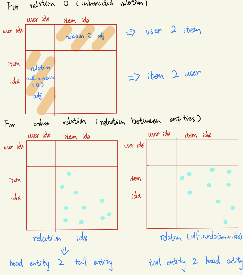
regard interacted as relation 0, now the number of relations is \(self.n\_relations+1\)
every relation \((idx)\) convert to 2 adjacency matrix (by inversing cols and rows), which representate as 2 new relations \((idx, self.n\_relations+idx)\):

As a result: we get adj_list, adj_r_list
1 | adj_list: [adjancy matrix1, adjancy matrix2,adjancy matrix3,...] |
Than, genarate adjancy matrix after laplacian normalization and save in self.lap_list.
Update kg dict
according to the change of relation, update kg dict
Generate batch data
build_model
Placeholder definition
1 | def _build_inputs(self): |
trainable weight definition
1 | def _build_weights(self): |